
Continuation-Extension of EOM Stock-Bond-Reversal Strategy
Part 2 of Profiting from Predictable Money Flows

This is part 2 of my “Profiting from Predictable Money Flows Series”. Here you will find Part 1.

A short recap, the EOM strategy invests in the early in the month underperformer for the last trading days because there is a reversal effect due to rebalancing by institutional investors.
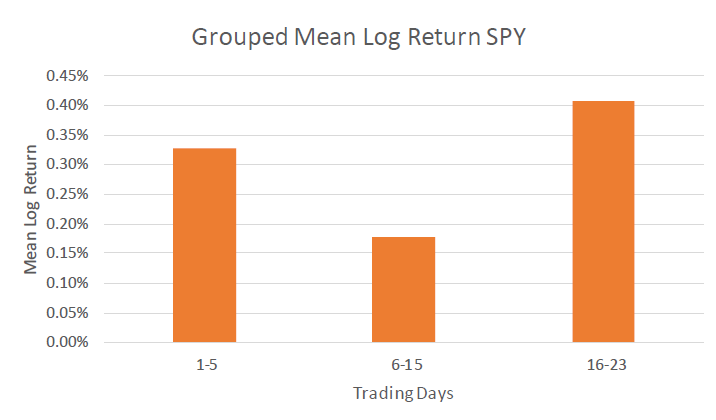
As shown in my previous post, SPY historically posts its strongest average gains in the closing days of the month, with the early-month period coming in second. Figure 1 provides a visual breakdown of this pattern.
To dig deeper, I looked at whether the strength or weakness of the first half of the previous month has any bearing on what comes next. In other words, does SPY tend to perform better when the first 15 trading days of the prior month were strong or weak? Figure 2 shows the results.
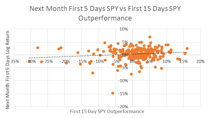
A clear pattern emerges when looking at the data: how SPY performs in the first half of a month often foreshadows what will happen at the start of the next one. If the initial 15 trading days are strong, the market typically carries that momentum into the first week of the following month. But if the early-month performance is weak, the next month’s opening days often follow suit.
In conclusion, the monthly cycle of SPY appears to break into three meaningful phases. The first 15 trading days serve as a trend-setting period that often signals the market’s underlying direction. The final 5 trading days typically represent a reversal window, where performance frequently diverges from the earlier trend due to the rebalancing effect. Then, as the new month begins, the first 5 trading days commonly resume the trend established during the initial half of the previous month.
Here’s the hypothesis:
This extension of the original EOM strategy will improve returns because we are longer invested and can harness the equity risk premium and the continuation effect (sort of momentum).
Testing the Theory
To test the hypothesis, the analysis uses two liquid ETFs:
SPY – S&P 500 ETF as a proxy for equities
TLT – 20+ Year U.S. Treasury ETF as a proxy for bonds
A typical month includes 20–23 trading days. The strategy examines performance during:
First 15 trading days → to identify the outperformer
Final 5–8 trading days → to capture potential reversal from rebalancing
First 5 trading days next month→ to capture potential continuation effect
Trading Setup
The execution of the strategy is refreshingly simple:
Around the 15th trading day, determine which asset outperformed since the start of the month.
Position for reversal:
If SPY outperformed TLT, go long TLT.
If TLT outperformed SPY, go long SPY.
Hold until month-end, then close the position.
If SPY outperformed TLT in the first 15 trading days, go long SPY at the start of next month.
Hold until trading day no. 5, then close the position.
Repeat each month.
As with the original end-of-month strategy, precise timing isn’t required—and realistically, it isn’t achievable. The approach relies on broader patterns rather than pinpointing exact days.
The Results
In the next figure, you can see how this EOMC (end of month + continuation) strategy performs year by year. The idea is straightforward: during the final five trading days, take a long position in the asset that underperformed earlier in the month. Then, if SPY outperformed TLT over the first 15 trading days, switch to a long SPY position for the first five days of the next month.
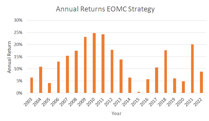
Over the 20-year sample period, the strategy delivered a compound annual growth rate (CAGR) of 12.34%, indicating strong and consistent long-term performance. Notably, the strategy avoided negative annual returns at any point during the sample, suggesting that its underlying approach can withstand market variability. The period immediately after the financial crisis proved especially favorable, yielding some of the strategy’s strongest annual results. However, in the last several years, performance has shown greater fluctuations and has not matched the stability observed during the earlier part of the sample period.
It is critical to acknowledge that, despite the absence of negative yearly returns within the given sample period, such an outcome should not be viewed as indicative of future performance trends. The only reasonable course of action is to expect that negative years can and will occur in the future.
Figure 4 presents a comparison of the cumulative performance of the EOMC strategy versus SPY, allowing for a straightforward assessment of how the strategy has performed relative to the market benchmark over time.
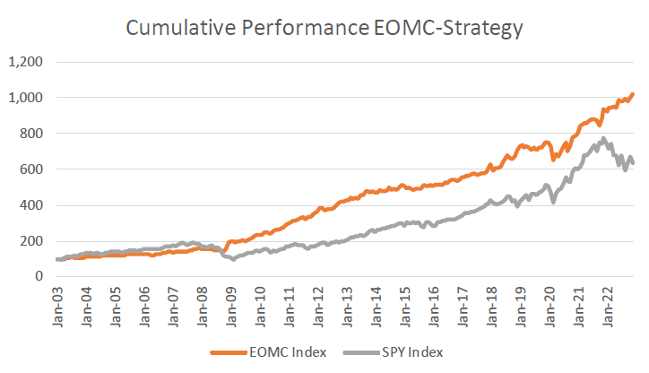
Prior to 2008, SPY exhibited superior cumulative performance relative to the EOMC strategy. Following the onset of the post-crisis recovery in 2009, this relationship inverted, with the EOMC strategy demonstrating sustained outperformance over SPY throughout the subsequent period.
The EOMC strategy constitutes a methodological advancement over the original EOM strategy. Empirically, it achieves higher absolute performance, and its expected Sharpe ratio of 1.00 indicates an improved risk-adjusted return profile.
Conclusion
The extended EOMC strategy works by taking advantage of a series of predictable monthly market behaviors: the tendency to reverse near the end, and to continue moving in the direction of prior momentum. By combining these phases into a single rules-based model, the strategy effectively captures the impact of institutional investors adjusting their portfolios.
What makes this approach appealing is not only that it boosts returns but that it does so with impressive steadiness. Over the last twenty years, the EOMC strategy generated a strong double-digit annual growth rate and did not experience a single losing year, clearly outperforming SPY. Even though the most recent period has produced more mixed results, the main force driving the return (structural market flows) remains in place.
Overall, the EOMC approach shows that monthly patterns in the market offer useful information. By extending the original end-of-month reversal idea to include early next month trends as well, investors gain access to a more dependable and diversified source of performance.
In part 3, I’ll unveil an extended version of this strategy that introduces shorting which will boost the expected Sharpe ratio up to 1.37.
Thank you for your interest in this post. If you liked it, I would really appreciate a like, as these are very motivating.
You are also welcome to share this post with others.
Disclaimer
The above article constitutes my or the authors’ personal views and is for entertainment purposes only. It is not to be construed as financial advice in any shape or form. Please do your own research and seek your own advice from a qualified financial advisor. I / The authors may from time to time hold positions in the aforementioned securities consistent with the views and opinions expressed in this article. The information provided in this article is not making promises, or guarantees regarding the accuracy of information supplied, nor that you guarantee for the completeness of the information here. The information in this article is opinion-based and that these opinions do not reflect the ideas, ideologies, or points of view of any organization the authors may be potentially affiliated with. The authors reserve the right to change the content of this blog or the above article. The performance represented is historical and that past performance is not a reliable indicator of future results and investors may not recover the full amount invested.