Volatility Decay Capturing

How to Benefit from Daily Market Fluctuations

This is the first of several posts about a strategy to capture the decay in leveraged ETFs. This is the undisclosed strategy from my last portfolioupdate.

One of the more counterintuitive strategies involving leveraged exchange-traded funds (LETFs) is to short both a leveraged ETF and its corresponding inverse ETF counterpart at the same time. At first glance, this seems illogical. If one fund is designed to profit when the underlying index rises and the other profits when it falls, how can betting against both possibly make sense?

The answer lies in a characteristic of leveraged ETFs known as volatility decay (this effect has many names, e.g. volatility drag or variance drain). This effect causes both the bullish and bearish versions of leveraged ETFs to gradually lose value over time when the underlying asset experiences significant price fluctuations, even if it ultimately goes nowhere.

What Is a Leveraged ETF?

A leveraged ETF is an exchange-traded fund designed to deliver a multiple of the daily return of an underlying asset. Unlike traditional ETFs, which aim to track the performance of an index on a one-to-one basis, leveraged ETFs amplify daily price movements through the use of derivatives.

Common leverage ratios include:

• 2x (twice the daily return)

• 3x (three times the daily return)

• –1x, –2x, and –3x (inverse leveraged ETFs that move in the opposite direction)

For example, a 3x S&P 500 ETF aims to generate three times the daily return of the S&P 500 Index. If the index rises by 1% during a trading day, the ETF seeks to gain 3%. Conversely, if the index falls by 1%, the ETF loses 3%.

The important word here is daily. Leveraged ETFs reset their exposure at the end of every trading day. As a result, their long-term performance is not simply three times the cumulative return of the underlying index! Instead, their returns become highly dependent on the path that prices take over time.

---

---

Understanding Volatility Decay

Volatility decay is the gradual erosion of value caused by the daily compounding of leveraged returns. When markets fluctuate back and forth, gains and losses are applied to an ever-changing portfolio value, causing leveraged ETFs to lose value over time even when the underlying index finishes unchanged.

Consider the following example:

Suppose an index starts at 100.

• Day 1: The index rises 10%, increasing from 100 to 110.

• Day 2: The index falls 9.09%, returning from 110 back to 100.

After two days, the index has ended exactly where it started. An investor holding the index would have neither gained nor lost money.

Now consider a 3x leveraged ETF tracking that same index.

• Day 1: The ETF gains 30%, rising from 100 to 130.

• Day 2: The ETF loses 27.27% (three times the index’s 9.09% decline), falling from 130 to approximately 94.55.

Although the underlying index is unchanged, the leveraged ETF has lost 5.45% of its value.

This loss is not due to poor tracking or management, it is a direct consequence of daily leverage and compounding. This phenomenon is known as volatility decay. The higher the leverage the higher the decay.

Why Both the Bull and Bear ETFs Lose Value

Both rebalance their leverage every day, and both experience the negative effects of compounding during volatile markets. As prices swing higher and lower, repeated gains and losses gradually reduce the value of both products over time.

This means that during periods of high volatility with no sustained trend, it is possible for both the 3x leveraged ETF and the 3x inverse ETF to decline simultaneously, even though they move in opposite directions on a day-to-day basis.

Why Traders Short Both ETFs

Because both leveraged ETFs tend to lose value over time due to volatility decay, traders attempt to capture this erosion by shorting both the long and inverse versions simultaneously. Both products decay, a short position in each should (in theory) profit purely from that decay. By doing this you’re not betting on the direction of the market. You’re betting purely on the mathematical drag baked into these leveraged products.

The strategy tends to work best when markets are sideways, range-bound or highly volatile without a clear long-term trend. In these conditions, volatility decay can accumulate rapidly, causing both ETFs to lose value.

Why It’s Not Free Money

Even if the strategy is market neutral it comes with real risks and costs:

• Trending markets hurt you. Volatility decay is strongest in choppy markets. In a strong (sustained) trend the winning leveraged ETF can rise faster than the losing one falls, leaving your combined short position with a loss. A powerful rally can send the 3x bull ETF soaring.

• Rebalancing is required. As one ETF rises and the other falls, your position sizes drift out of balance, re-exposing you to directional risk. Maintaining neutrality means periodically rebalance the two, which incurs transaction costs.

• Borrow costs and availability. Shorting requires borrowing shares. Leveraged ETFs can carry high borrow fees or can be hard-to-borrow/unborrowable. These shares may be recalled at inconvenient times.

• Margin and short squeezes. A sharp move in either LETF can trigger margin calls.

• Dividends and expense drag. You may owe any distributions on shares you’ve shorted, offsetting some of the decay you’re trying to capture.

Leverage Isn’t Automatically Bad

Leveraged ETFs often receive criticism because of volatility decay, but it is important to understand that leverage itself is not inherently harmful. Leverage simply increases both potential returns and potential risk. Whether a leveraged ETF is “good” or “bad” depends on how its level of leverage compares to the characteristics of the underlying asset.

To understand this, consider an unleveraged ETF and a leveraged ETF with a leverage factor of 3x.

If the underlying ETF has an annualized volatility of 20%, then a 3x leveraged ETF would be expected to have a volatility of approximately 60%. In other words, volatility scales linearly with leverage:

• Unleveraged ETF: 20% volatility

• 2x leveraged ETF: approximately 40% volatility

• 3x leveraged ETF: approximately 60% volatility.

This relationship is completely expected.

The existence of volatility decay does not automatically mean that every leveraged ETF is a good candidate for shorting. What ultimately matters is whether the ETF’s leverage is greater than the level that would maximize long-term compounded growth. When leverage exceeds this optimal level, the additional volatility creates more drag than the extra exposure can compensate for, leading to a gradual erosion in long-term performance. This is the type of ETF that tends to exhibit the strongest decay.

In other words, the relationship is not as simple as:

More leverage = more decay = better short

This is an interesting topic in its own right and is beyond the scope of this post. It deserves a dedicated discussion.

From Theory to Practice

Understanding volatility decay is one thing, designing a strategy that consistently captures it is another.

To illustrate the practical considerations, consider the following QQQ “ETF-family”:

• QQQ – Nasdaq-100 ETF

• TQQQ – 3x leveraged Nasdaq-100 ETF

• SQQQ – 3x leveraged inverse Nasdaq-100 ETF

The first challenge is constructing a position that is as close to market neutral as possible. Two common approaches are available.

Option 1: Short Both TQQQ and SQQQ

The most intuitive strategy is to short both the bullish and bearish leveraged ETFs simultaneously. Because both ETFs experience volatility decay, this approach attempts to capture the decay from both sides of the trade.

At first glance, this appears ideal. However, maintaining market neutrality is more difficult than it seems.

Imagine that the Nasdaq enters a strong bull market.

• TQQQ grows, so your short in it grows larger as a share of your portfolio.

• SQQQ shrinks, so your short in it shrinks.

The portfolio gradually develops a net short exposure to the market. If the rally continues, losses on the growing TQQQ short can easily exceed the gains generated by the shrinking SQQQ position.

The opposite occurs during a prolonged bear market.

For this reason, traders must periodically rebalance both positions to restore market neutrality. Rebalancing, however, is not free. It introduces transaction costs and potentially tax consequences, all of which reduce the profits generated by volatility decay.

This strategy behaves much like being short gamma. Large directional moves are harmful because they create increasingly unbalanced positions, while frequent back-and-forth price oscillations tend to be beneficial because they accelerate volatility decay.

Option 2: Short TQQQ and Long QQQ

An alternative approach is to short the leveraged ETF while simultaneously buying the unleveraged ETF.

Since TQQQ targets three times the daily return of QQQ, a common starting point is a 3:1 hedge ratio, holding roughly three dollars of QQQ for every one dollar short in TQQQ.

Compared with shorting both leveraged ETFs, this approach offers several advantages. The directional hedge is explicit and generally more stable, making the portfolio’s market exposure easier to understand and manage. It also avoids the continuously changing balance between two leveraged products that naturally occurs in the first approach.

The primary disadvantage is capital efficiency. A 3:1 hedge ratio requires substantially more capital because each dollar of TQQQ sold short must be offset by approximately three dollars invested in QQQ.

Choosing Between the Two Approaches

Neither implementation is universally superior. Ultimately, the best choice depends on the trader’s objectives and constraints.

The Results

The following chart presents the annual returns of both versions.

Figure 1: Annual Returns Short SQQQ+TQQQ & Short TQQQ + Long 3x QQQ Log return; index results, not achievable in reality

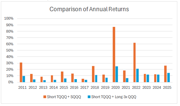
Both versions consistently generated positive annual returns before accounting for transaction costs and borrow fees. In practice, borrow fees will have a substantial impact on profitability. Therefore, the reported results should be interpreted as an indication of the strategies’ underlying performance rather than their expected realized returns.

Table 1: Performance overview; index results, not achievable in reality

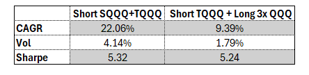
The Sharpe ratios reported for both versions should be interpreted with caution. Since the analysis does not incorporate borrow fees the reported returns are overstated. As a result, the corresponding Sharpe ratios are also inflated and should not be regarded as representative of the strategies’ real-world risk-adjusted performance. In real-world trading the Sharpe ratios will be significantly lower.

Despite this limitation, the comparison between the two versions remains informative. Version 2 exhibits lower volatility while achieving a Sharpe ratio that is approximately the same as that of Version 1. Version 2 will be less impacted by trading costs and borrow fees, so this suggests that it is likely to retain a stronger risk-adjusted profile once realistic trading costs are incorporated.

Key Takeaways

• This is a market-neutral strategy in theory, not always in practice. The trade is designed to profit from decay rather than direction, but it behaves like being short gamma, sideways/choppy markets help it, while strong sustained trends hurt it.

• Rebalancing is unavoidable and costly. As the market moves, position sizes drift out of balance, reintroducing directional exposure. Restoring neutrality requires periodic rebalancing, which adds transaction costs and tax consequences.

• Real-world costs significantly erode returns. Borrow fees and dividend obligations on shorted shares cut into the theoretical decay profits.

Conclusion

Volatility decay isn’t a bug, it’s the byproduct of daily compounding applied to leveraged exposure. In choppy, directionless markets, that decay is real and can be captured. But trending markets, rebalancing costs and borrow fees all chip away at the theoretical edge.

The comparison between shorting both TQQQ and SQQQ versus shorting TQQQ against a long QQQ position illustrates that there’s no single correct way to implement this idea. Each approach carries its own tradeoffs between capital efficiency, stability, and sensitivity to real-world frictions. The backtested results presented here are a useful starting point for understanding the underlying behavior of these strategies, but they should not be mistaken for a realistic estimate of achievable returns. Borrow costs alone will meaningfully change the picture.

For now, the key lesson is this: volatility decay is real, but capturing it profitably requires far more nuance than simply shorting LETFs and waiting.

---

Disclaimer

The above article constitutes my or the authors’ personal views and is for entertainment purposes only. It is not to be construed as financial advice in any shape or form. Please do your own research and seek your own advice from a qualified financial advisor. I / The authors may from time to time hold positions in the aforementioned securities consistent with the views and opinions expressed in this article. The information provided in this article is not making promises, or guarantees regarding the accuracy of information supplied, nor that you guarantee for the completeness of the information here. The information in this article is opinion-based and that these opinions do not reflect the ideas, ideologies, or points of view of any organization the authors may be potentially affiliated with. The authors reserve the right to change the content of this blog or the above article. The performance represented is historical and that past performance is not a reliable indicator of future results and investors may not recover the full amount invested.