


I published this post last week in German. As an experiment I am republishing it in English now. I will maybe publish more posts in English in the future. Let me know if you like it and be interested in more.
As previously announced, I have shifted my focus to quantitative investing. My current strategy is presented below, but it is still a work in progress and will see some adjustments. The strategy includes the three factors value, momentum and quality, and is also long-only. It combines all these factors, so it is not a portfolio of three strategies (one for each factor). I quite arrogantly call the strategy Holy Trinity. The individual factors are presented in more detail below.
Value
The value factor is not represented by one key ratio, but by a value composite. O'Shaughnessy (2012) and Carlisle and Gray (2013) have already demonstrated the advantages of a value composite over an individual key ratio. The main advantage is that the system is more robust against outliers. The value composite used consists of the following four ratios:
EBIT/EV
B/M
EV/S
GPA (Gross Profit/Total Assets).
The mix of ratios should be as broadly diversified as possible. The individual ratios have been selected deliberately.
EBIT/EV is selected as this corresponds to the acquirer's multiple, the effectiveness of which has been proven by Carlisle (2017), Schwarz and Hanauer (2024) and my own tests.
The B/M ratio (book to market) is the classic academic value ratio and differs fundamentally from the other ratios, as it does not use a figure from the income statement, but one from the balance sheet.
According to the third edition of O'Shaughnessy's “What works on Wall Street” (2005), P/S is the ratio with the best performance. Since I prefer the enterprise ratios, P/S has been changed to EV/S.
The Value Composite is rounded off by GPA (GP/TA), which is known from the work of Novy-Marx (2010). However, it does not seem to me to be very widespread, partly based on the download figures for the paper. However, Carlisle and Gray (2013) show the benefits of this indicator. Since gross profit is independent of the capital structure, it makes sense to use total assets as the denominator. Overall, however, the ratio is more like a quality ratio than a value ratio.
It cannot be ruled out that my Value Composite will be supplemented by other key figures. Free cash flow, for example, is a very prominent value indicator that is missing.
To determine the Value Composite, the key figures are first considered individually, each key figure is ranked individually and at the end (the ranks) are added up to an overall value. The higher the overall value, the better.
Momentum
The momentum factor is currently considered to be the performance of the share price over the last 12 months. This must be positive. It is therefore a time-series momentum indicator. In academic publications, the most recent month is normally left out. I will probably switch to this approach in the long run.
Quality
The FS-Score by Carlisle and Gray (2013), which is an adaptation of the Piotroski F-Score, is used as a quality indicator. A separate article will be published on the comparison of F- and FS-Score (In German and maybe afterwards in English). Only shares with a value >= 8 are considered. The 10 key figures of the FS-Score cover a broad spectrum of quality indicators; accordingly, no other quality indicators are considered.
Selection
Similar to the Piotroski F-Score or the FS-Score by Carlisle and Gray (2013), shares are ranked according to the value component. The selected factors complement each other well, as value and momentum are negatively correlated, as are quant value and quality. If value is used alone, there is a risk of investing in value traps. Momentum provides a catalyst, so to speak, as the market has become aware of the share and has recognized it's potential, at least to some extent (Petersen 2015). The quality factor further reduces the risk of a value trap. Ultimately, this strategy involves buying shares that are in an upward trend and are relatively cheap for their quality level.
Backtesting
The backtests are based on data from Portfolio123. It cannot be ruled out that the results are distorted by survivorship bias and look-ahead bias. Transaction costs, taxes and other practical characteristics are not taken into account, as the results relate to indices that are not directly investable. The data and calculation methods used may contain inaccuracies or errors and certain assumptions have been made which may differ in reality. The results may vary depending on the data source selected. The observation period is 16 years from 01/01/2009 to 12/31/2024. Such a period is too short to make valid statements about the long-term performance of the strategies presented.
The results are first presented for the P50 portfolios (50 shares) and then for the P25 portfolios (25 shares). Figure 1 shows the development of the cumulative performance of the individual P50 portfolios at different rebalancing cycles 52 weeks, 26 weeks and 13 weeks.

The outperformance of the 52W and 26W portfolios is clearly recognizable, as is the underperformance of the 13W portfolio, whose underperformance does not begin until 2020.
Table 1 lists the individual key figures for the variants (portfolios).
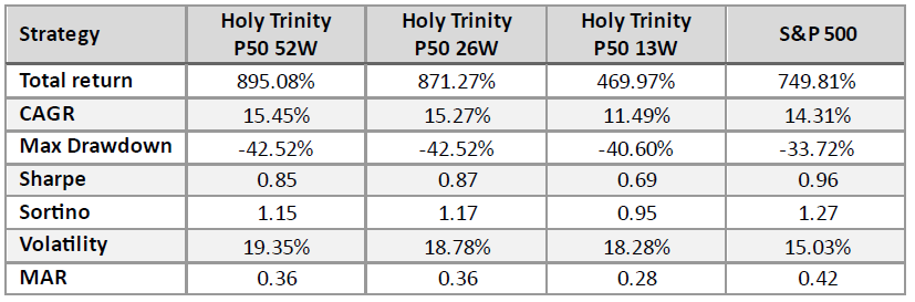
The 52W and 26W portfolios outperform the S&P 500. The 13W portfolio significantly underperforms the S&P 500.
The S&P 500 has the lowest maximum loss (-33.72%) and the lowest volatility (standard deviation). The Holy Trinity portfolios have higher losses (up to -42.52 %) and higher standard deviations (18.28 % - 19.35 %). However, the standard deviations are still very low for portfolios with 50 stocks.
The S&P 500 Index has the best Sharpe, Sortino and MAR ratios. The Holy Trinity portfolios have lower, but still very good risk/return ratios.
Figure 2 shows the development of the cumulative performance of the individual P25 portfolios.

The outperformance of the 52W portfolio is clearly visible. The other two portfolios achieved the same performance as the S&P 500 until 2019, but have lagged behind since then.
The 52W portfolio achieves the highest total return/CAGR and outperforms the S&P 500. The other two variants lag well behind the S&P 500.
Table 2 lists the individual key figures for the variants (portfolios).
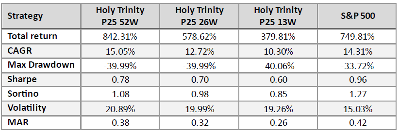
The 52W portfolio outperforms the S&P 500, while the other two underperform it. The maximum loss is almost identical for all Holy Trinity portfolios and slightly higher than for the S&P 500. The standard deviations are very low for portfolios with 25 stocks.
The S&P 500 Index has the best Sharpe, Sortino and MAR ratios. The Holy Trinity portfolios have lower, but still very good risk/return ratios.
Summary of the backtest
For P50 and P25 portfolios, the return decreases the more often the rebalancing or recalculation is carried out. No portfolio comes close to the risk-adjusted return of the S&P 500. Surprisingly, the maximum losses in the more broadly diversified P50 portfolios are larger than in the P25 portfolios. Volatility is lower for P50 portfolios, as you would expect.
A few words on the performance of the S&P 500 to put it into context. It has achieved an annual return of 14.31 %. This is a very good return and well above historical levels. By comparison, the compound annual growth rate (CAGR) from 1964 to 2011 was 9.52 % (Gray and Carlisle 2013). The Sharpe and Sortino ratios are also exceptionally good at 0.91 and 1.22 respectively. By way of classification: Sharpe ratios at or above 0.50 can be classified as good, especially in a portfolio context (Kestner 2014). These good results are mainly due to the lack of market corrections. Outside of the pandemic, there was no major market correction during the period under review.
Portfolio structure
The portfolio has an international structure. At the start, it consists of the USA, the UK and Germany. The initial breakdown is 50% USA, 25% UK and 25% Germany. The US strategy consists of 48 stocks and 24 each for the UK and Germany. Other countries will be added in the future.
However, the shares are not all bought at the same time, but the 4 best shares for the US and the best 2 shares in each of the other two countries are bought each month. These shares are then held for 12 months. This creates an overlapping portfolio. This procedure has the advantage that any changes to the strategy can be implemented directly in the following month. The rebalancing will initially take place with the sale and purchase after one year. However, rebalancing during the year will probably be implemented at a later date. There will be human intervention in the portfolio in the event of insolvencies, takeovers, delistings, etc.
Portfolio Update February
Buys
US-Portfolio
$VLGEA – Village Supermarket
$SGRP – SPAR Group
$SCG – Superior Group of Companies
$APEI - American Public Education
UK-Portfolio
$KGF – Kingfisher
$ECEL – Eurocell
GER-Portfolio
$EVK – Evonik Industries
$TUI1 – TUI
Thank you for your interest in this post. If you liked it, I would really appreciate a Like, as these are very motivating.
You are also welcome to share it with others.
Disclaimer
The above article constitutes my or the authors’ personal views and is for entertainment purposes only. It is not to be construed as financial advice in any shape or form. Please do your own research and seek your own advice from a qualified financial advisor. I / The authors may from time to time hold positions in the aforementioned stocks consistent with the views and opinions expressed in this article. The information provided in this article is not making promises, or guarantees regarding the accuracy of information supplied, nor that you guarantee for the completeness of the information here. The information in this article is opinion-based and that these opinions do not reflect the ideas, ideologies, or points of view of any organization the authors may be potentially affiliated with. The authors reserve the right to change the content of this blog or the above article. The performance represented is historical" and that "past performance is not a reliable indicator of future results and investors may not recover the full amount invested.